R Markdown

This post introduces our recently published R package, CIM, to measure the impacts of migration on local population structures. We developed the methodology in this paper in 2018. This paper is one of the top ten most viewed articles in Population Studies

Installing

install.packages("CIM")
library(CIM)

This package enables quantifying the impact of internal migration on age, gender, educational population structures and inequality.

Example

Here I provide a short example of how this can be used to measure the impact of internal migration on residential age segregation in the Greater London Metropolitan Area, England, drawing on one-year migration data by age bands (i.e. 1-14, 15-29, 30-34, 45-64 and 65+) at the local authority level, 2011 UK Censuses. Local authorities comprising outside the Greater London Metropolitan Area are collapsed into a single area, labelled “the Rest of the UK”. I use the same approach employed by Rodríguez-Vignoli and Rowe (2017) to measure the impact of internal migration on residential educational segregation in the Greater Santiago, Chile.

Computation

Compute and print the CIM outputs

CIM.duncan <- CIM(pop65over, pop1_14, pop15_29, pop30_44, pop45_64, calculation = "duncan", numerator = 1, DuncanAll = TRUE)
CIM.duncan$duncan_index
## [1] 0.02813039

Interpretation

The CIM for the Duncan index of dissimilarity indicates that internal migration has contributed to increase age segregation of the population aged 65 and over in the Greater London Metropolitan Area by 2.81% between 2010 and 2011 i.e. from 16.2% in 2010 to 19% in 2011.

Visualisation

To visualise where the population aged 65 and over in the Greater London Metropolitan Area is concentrating, we can map differences in the spatial distribution of this population across local authority districts.

First install and load the needed packages

install.packages(c("sf", "dplyr", "ggplot2", "viridis"))
library(sf)
library(dplyr)
library(ggplot2)
library(viridis)

NOTE: Download a shapefile containing the Greater London Local Authority Districts from the shapefile folder from this github repository

NOTE: The Local Authority Districts for the City of London and Westminster in our shapefile are combined to make our shapefile consistent with our migration data.

Read the shapefile.

library(sf)
shapefile_path <- file.path("shapefiles", "greater_london", "Greater_London_districts.shp")
if (!file.exists(shapefile_path)) {
  stop("Shapefile not found at: ", shapefile_path)
}
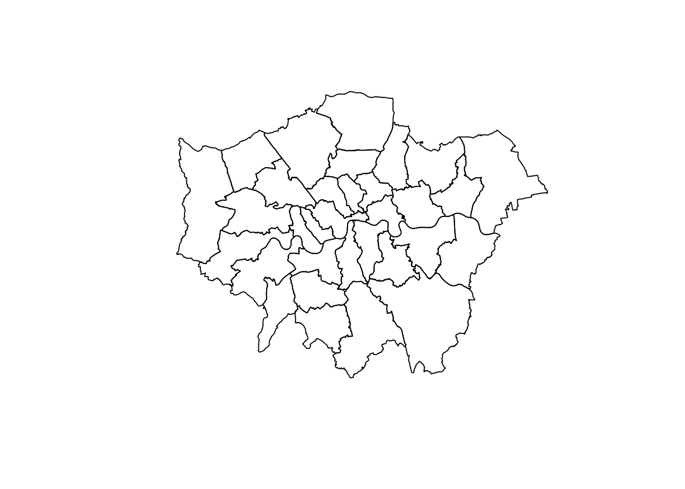
Greater_London <- st_read(shapefile_path, quiet = TRUE)

Plot the shapefile

ggplot(Greater_London) +
  geom_sf(fill = "#f8fafc", colour = "#475569", linewidth = 0.2) +
  labs(title = "Greater London local authority boundaries") +
  theme_void(base_size = 11) +
  theme(
    plot.title = element_text(face = "bold", colour = "#111827", size = 12),
    plot.background = element_rect(fill = "white", colour = NA)
  )

Obtain the differences in the spatial distribution of the population aged 65 and over across local authority districts using the CIM.Duncan function:

CIM.duncan <- CIM(pop65over, pop1_14, pop15_29, pop30_44, pop45_64, calculation = "duncan", numerator = 1, DuncanAll = TRUE)
Dun_65over <- CIM.duncan$duncan_results

Visualise the results

head(Dun_65over)
##                      ASFVShare_cg ASCFVShare_cg ASFVShare_ref ASCFVShare_ref
## Barking and Dagenham   0.01745867    0.02110757    0.01722178     0.01758504
## Barnet                 0.06271777    0.05474050    0.03975623     0.03996727
## Bexley                 0.03017273    0.02974775    0.01669010     0.01719928
## Brent                  0.02998740    0.03487968    0.03538955     0.03798874
## Bromley                0.05326562    0.05218904    0.02702766     0.02666937
## Camden                 0.03054341    0.02879095    0.03624574     0.03625877
##                      ASShareFV_diff ASShareCFV_diff
## Barking and Dagenham   0.0002368912     0.003522525
## Barnet                 0.0229615445     0.014773235
## Bexley                 0.0134826294     0.012548474
## Brent                  0.0054021543     0.003109066
## Bromley                0.0262379625     0.025519669
## Camden                 0.0057023363     0.007467818

Append these data to the shapefile using the local authority names as joiner

library(dplyr)
dun_df <- data.frame(Dun_65over, name = rownames(Dun_65over), row.names = NULL)
dun_df <- subset(dun_df, name != "totalCol")
Duncan_65p <- left_join(Greater_London, dun_df, by = "name")
head(st_drop_geometry(Duncan_65p))
##   label                 name ons_label ASFVShare_cg ASCFVShare_cg ASFVShare_ref
## 1  02AF              Bromley      00AF   0.05326562    0.05218904    0.02702766
## 2  02BD Richmond upon Thames      00BD   0.03117355    0.03061757    0.02315899
## 3  02AS           Hillingdon      00AS   0.03495441    0.03511163    0.02920845
## 4  02AR             Havering      00AR   0.03873527    0.03308205    0.01642682
## 5  02AX Kingston upon Thames      00AX   0.02153607    0.02244129    0.02197114
## 6  02BF               Sutton      00BF   0.02869004    0.02681937    0.01560226
##   ASCFVShare_ref ASShareFV_diff ASShareCFV_diff
## 1     0.02666937   0.0262379625     0.025519669
## 2     0.02254429   0.0080145627     0.008073282
## 3     0.02856140   0.0057459601     0.006550226
## 4     0.01652916   0.0223084481     0.016552889
## 5     0.02044645   0.0004350701     0.001994836
## 6     0.01630248   0.0130877815     0.010516890

Create a map using ggplot.

plot_data <- Duncan_65p |>
  filter(!is.na(ASShareFV_diff))

map_labels <- bind_rows(
  slice_max(plot_data, ASShareFV_diff, n = 1, with_ties = FALSE),
  slice_min(plot_data, ASShareFV_diff, n = 1, with_ties = FALSE)
) |>
  mutate(
    label = paste0(
      if_else(ASShareFV_diff == max(plot_data$ASShareFV_diff), "Highest: ", "Lowest: "),
      name,
      "\n",
      round(ASShareFV_diff * 100, 2),
      " percentage points"
    )
  )
label_points <- suppressWarnings(st_point_on_surface(map_labels))

ggplot(plot_data) +
  geom_sf(aes(fill = ASShareFV_diff), colour = "white", linewidth = 0.18) +
  geom_sf_label(
    data = label_points,
    aes(label = label),
    size = 3,
    linewidth = 0.2,
    label.padding = unit(0.18, "lines"),
    fill = "white",
    colour = "#1f2937"
  ) +
  scale_fill_viridis_c(
    option = "viridis",
    labels = scales::label_percent(accuracy = 0.1),
    name = "Change in share"
  ) +
  labs(
    title = "Internal migration and age segregation in Greater London",
    subtitle = "Difference in the local share of the population aged 65+ attributable to migration",
    caption = "Source: CIM package example data and Greater London local authority boundaries."
  ) +
  theme_void(base_size = 12) +
  theme(
    plot.title = element_text(face = "bold", colour = "#111827", size = 14),
    plot.subtitle = element_text(colour = "#4b5563", size = 10, margin = margin(b = 10)),
    plot.caption = element_text(colour = "#6b7280", size = 9, hjust = 0),
    legend.position = "right",
    legend.title = element_text(face = "bold", size = 10),
    legend.text = element_text(size = 9),
    panel.background = element_rect(fill = "#f8fafc", colour = NA),
    plot.background = element_rect(fill = "white", colour = NA),
    plot.margin = margin(8, 10, 8, 10)
  )

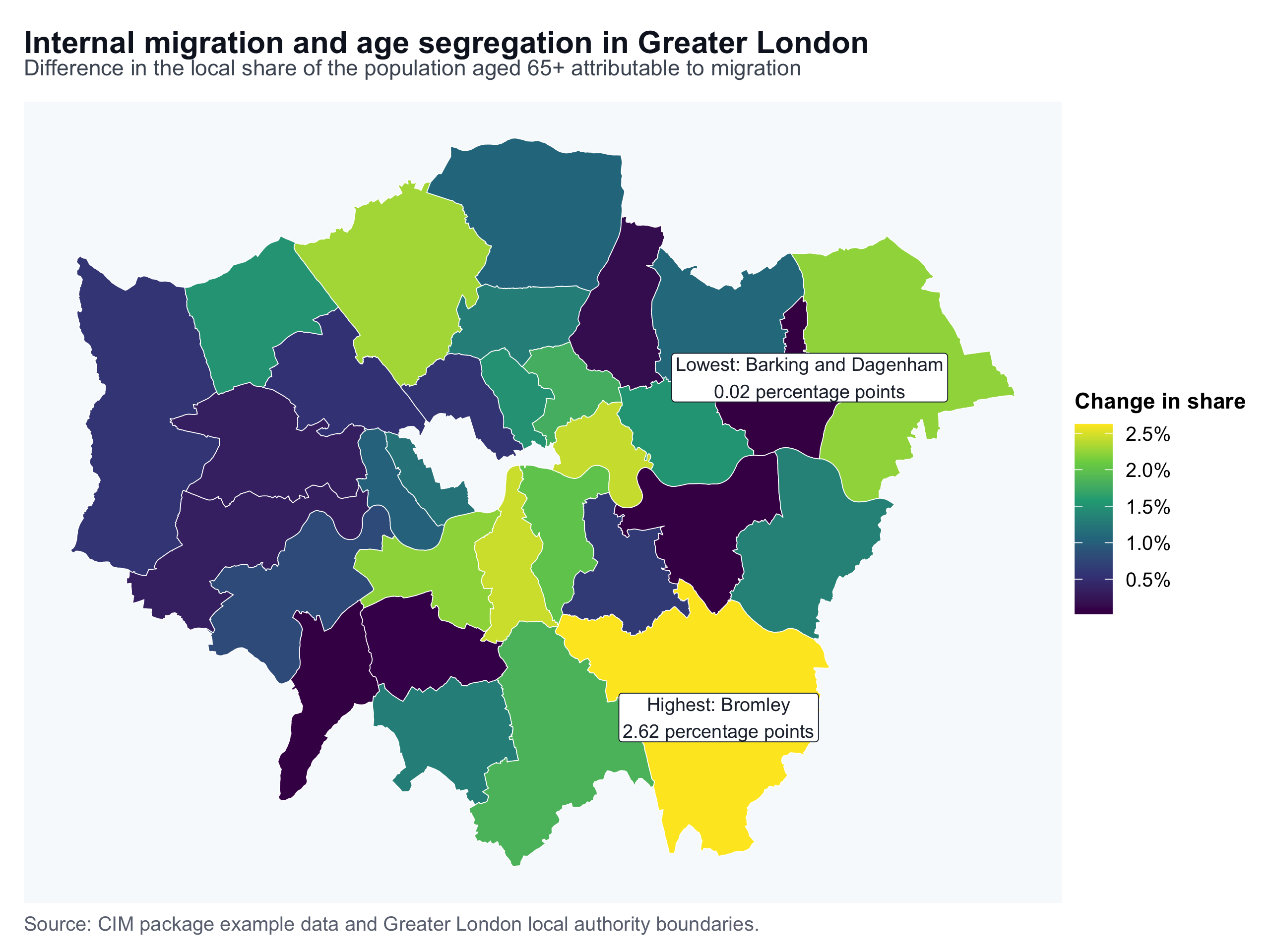
Migration had the largest estimated contribution to the concentration of residents aged 65+ in Bromley (2.62 percentage points), while the smallest contribution was in Barking and Dagenham (0.02 percentage points).

References

Rodríguez-Vignoli, Jorge, and Francisco Rowe. 2018. “How is internal migration reshaping metropolitan populations in Latin America? A new method and new evidence.” Population Studies 72 (2): 253-273. https://doi.org/10.1080/00324728.2017.1416155

Introducing the R Package CIM